Multi-Touch Attribution, or MTA, seeks to better understand what truly drove or “caused” an action to happen. How does multi touch attribution work? Usually, these actions are online and commercial in nature. The most typical use case is understanding what drove an order or a transaction. These “part-worths” can then be summed up across many orders or transactions to form a complete picture of how different marketing channels contributed to the sales accrued in a given period.
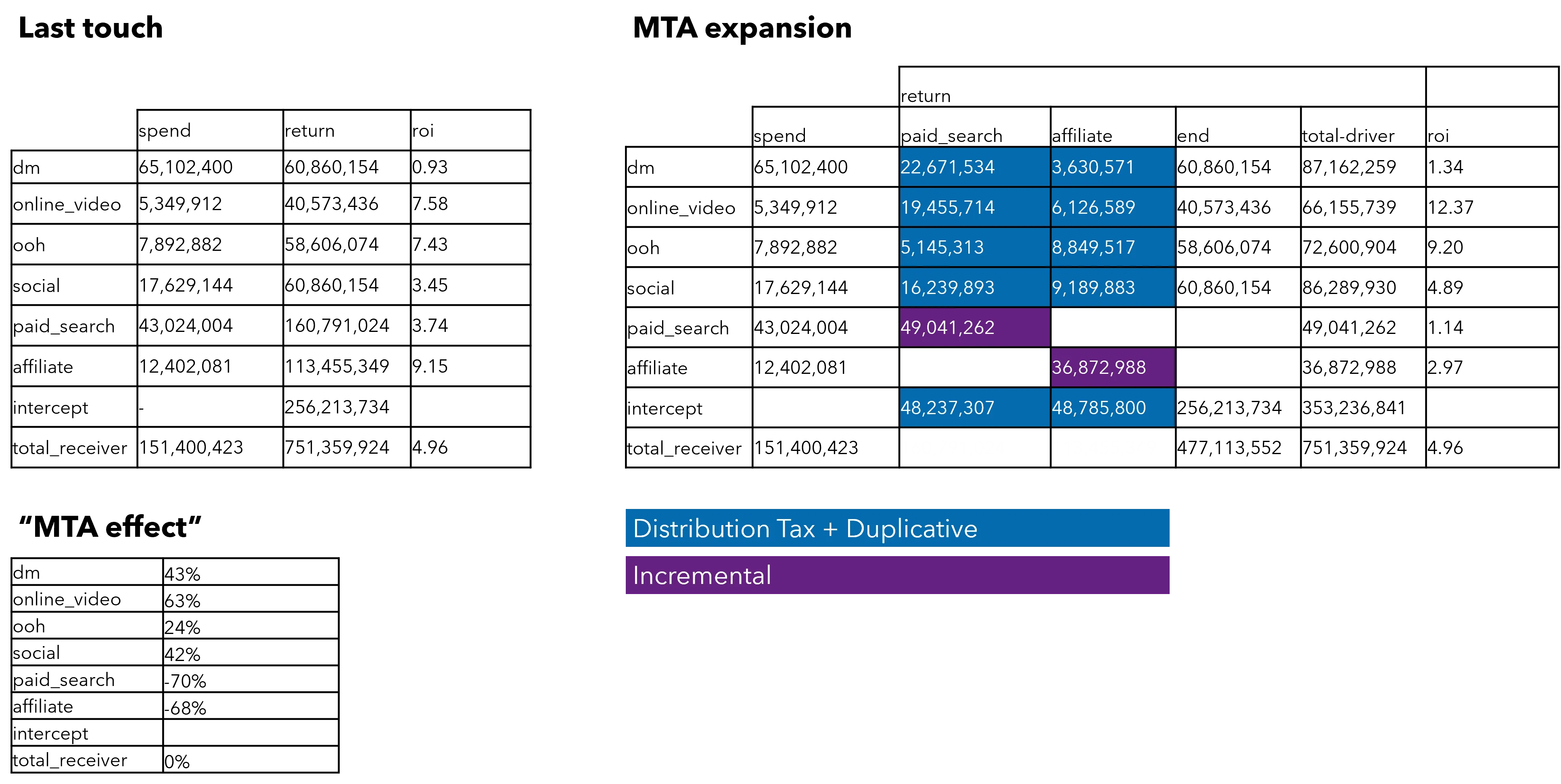
For example, say a user purchased a subscription to a monthly ride-sharing service. It is easy to know that the user entered from a paid search ad; each ad has a unique referring URL that can be tracked. However, giving all credit to the paid search ad is most likely unfair. The user might have seen a social media campaign days before, or an ad on a baseball game weeks before. Those touches should also receive credit. The difference between a last-touch and multi-touch attribution is usually substantial. Lower-funnel channels usually look less attractive in a multi-touch approach (see Figure 1 below).

Figure 1: A last-touch versus a multi-touch approach can yield very different results. The “MTA effect” shows less attractive results for paid search and affiliate, and better results for DM, online video, and social in this example.
To accurately apportion credit to all contributing channels, it is necessary to estimate the effect that each touch had on the customer who ultimately ordered. This requires, at the most basic level, knowing that a previous interaction occurred. This is the number one problem with multi-touch attribution: gathering the “touches”.
Historical Context of Tracking
In the first decade of the 2000s, tracking users across digital properties was easier. Customers’ browsers held records of where they had been and what they had done. These cookies functioned as digital breadcrumbs, alerting an advertiser that a consumer had seen an ad weeks before. It was possible for advertisers to piece together customer journeys deterministically—that is, knowing concretely when and what someone saw before they made an order. With these data censuses, early MTAs could estimate each touches’ effects simply—typically applying even credit to each touch, with linear decays of impact over time—or using more complex methods.
Privacy Measures Impacting MTA
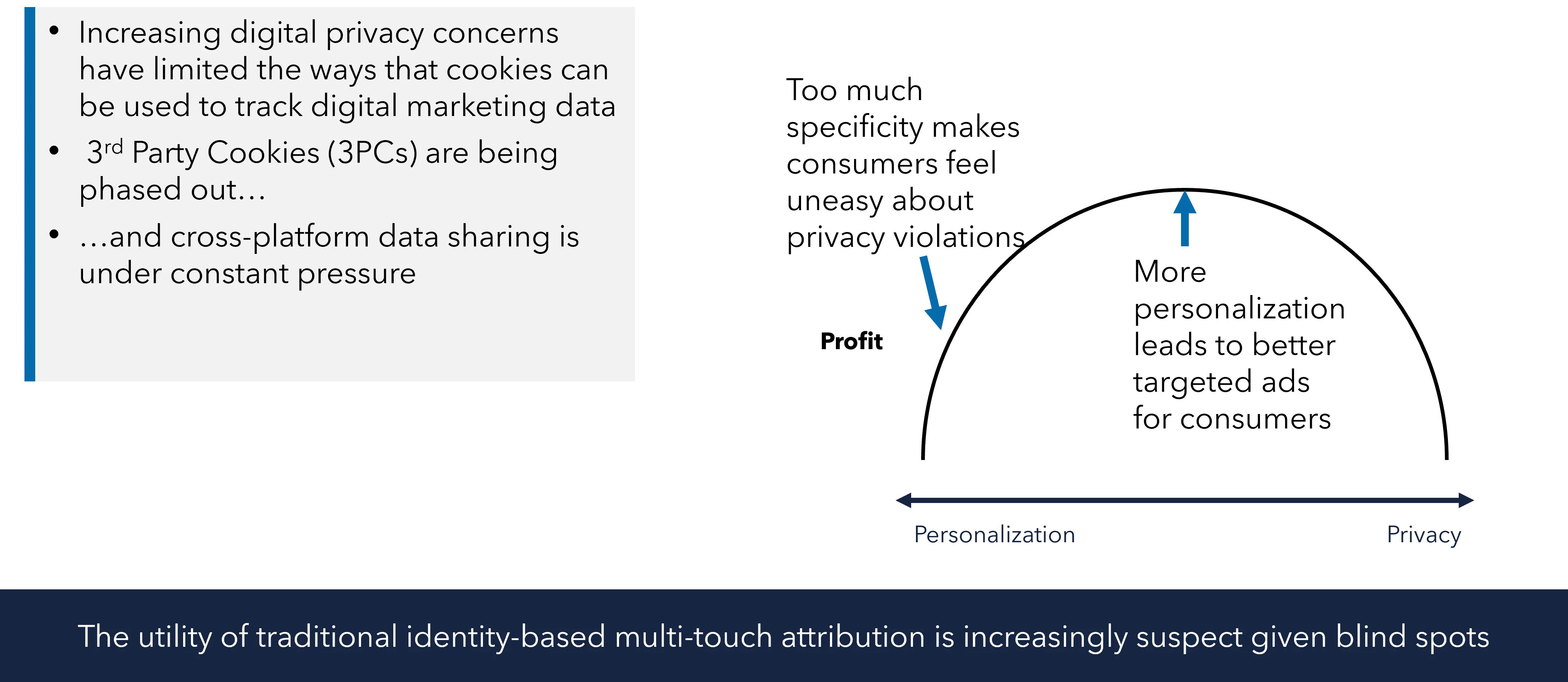
However, over the past several years, it has become more difficult to build truly deterministic MTAs. Privacy measures—whether cookie deprecation, walling off app data interchanges, or obfuscation of PII in third-party data sources—have made it harder and harder to say that a pageview or click was the result of an individual customer with any degree of confidence. The tradeoff between privacy and customization will likely be a forever war (see Figure 2)—suggesting an owned, decoupled approach to attribution that doesn’t rely on fads or black boxes.

Figure 2: The push and pull between privacy and personalization will likely be a forever war.
First-Party Data: The Advertiser’s Advantage
Some data sources are still totally knowable. Anything directly controlled by the advertiser—sometimes called first-party data—can be tracked in principle. Examples of these first-party interactions include email, direct mail, landing pages (or any web pages on the company website), owned or cooperative advertising networks, and call centers—whether customer support or acquisition-focused. In these cases, previous touches and interactions with an individual can be reconstructed as an identity graph, tied together with some unique ID.
Dealing with Unknown Identities
In most cases, however, interactions with customers are “underwater”—unknown to everyone but the individual and the publisher that he interacted with. In these cases, all hope is not lost. There are two basic approaches to dealing with resolving unknown identities.
Identity Resolution Technology
The first is using an identity resolution technology provider. These data brokers provide crosswalks between different walled gardens, by either inking proprietary sharing agreements or by using algorithms to match up individuals by using various pieces of their identity to build “fingerprints.” The fidelity of matching can vary from very low to approaching 50%—which is quite good. The trick is, most of these providers do not want to give up their raw data. Instead, they prefer to keep identities in their domain, for obvious reasons. In fact, most identity resolution providers’ first business is activation, not measurement. They provide value by essentially extending retargeting—the continued advertisement to one user over time—to broader parts of the digital domain.
Even so, it’s worth following up with a few vendors to see what they are willing to provide. In some cases, APIs may be provided that return a proprietary ID (or not) to a given third-party interaction. At scale—over millions of interactions—this approach can help build a deterministic identity graph.
Probabilistic Assignment of Interactions
Another approach is probabilistic assignment of interactions. This approach—while less precise than deterministic assignment of interactions—is also not vulnerable to future changes to platform privacy policies. In this framework, each identity (user) is assigned a probability of having seen an advertisement based on time and location.
For example, say we know that in the Memphis DMA on May 1st, there were 1,045 paid social ads served (these types of data are usually available from platforms, or via the digital agency executing the marketing.) The only other piece of data we would need would be the targeting criteria for the campaign (say, 18-34 year olds), and the number of those people in the DMA. From the American Community Survey (ACS), we know that the 2022 1-year estimates for 18-34-year-olds is 367,709 in the Memphis MSA (Metropolitan Statistical Area)—not an exact match for DMA but close enough. In that case, we can say that on May 1st, an 18-34-year-old individual in that area would have a 1,045 / 367,709 (0.28%) chance of having seen that ad.
This approach can work for virtually any media channel, from targeted to broad reach. It obviously is less accurate and contains significant potential error, but in aggregate, it is a powerful tool to create all encompassing media attribution.
Building a Longitudinal Human Record (LHR)
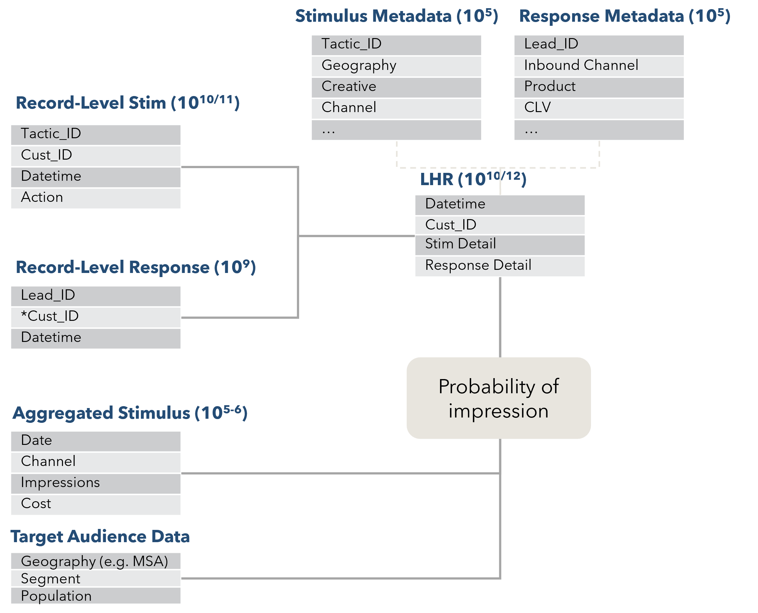
In reality, a mixture of discrete (identity resolved) and aggregated (estimated) impressions will be used in a comprehensive MTA (see Figure 3). Whatever the combination, the aim is to end up with a longitudinal human record (LHR)—the data structure also used for CDPs (customer data platforms.) This data structure in “tall and skinny”—in other words, it will have many rows and few columns. A typical LHR used for multi-touch attribution will have hundreds of millions or billions of rows, and something like 10-20 columns.

Figure 3: A mixture of record-level (deterministic) and aggregated (probabilistic) data sources to build the longitudinal human record (LHR)
The most important columns in the LHR are the date-time of the interaction in question and the ID of the “individual”. The records should be sorted first by ID, and then by date-time. In other words, all interactions associated with an ID x will be grouped together, and then sorted by date-time descending, with the most recent interaction at the top. In the case of an order—the thing you are trying to attribute in MTA—this will generally be at the top of a lot of previous interactions.
Apportioning Value to Interactions
Once the data are constructed, a method is required to apportion value to each of the previous interactions. The simplest method is equal apportionment—and it’s not necessarily a bad place to start. Say an ID associated with an order has 40 logged interactions in the prior 90 days. In this case, each of the 40 interactions would receive 1/40th of the credit for the order.
This simple method can be made more accurate by discounting “probabilistic” interactions by their probabilities. For example, in the case of the 0.28% chance someone in Memphis saw the social ad on May 1st above, that record would be a 0.0028 in both the numerator and the denominator of the attribution equation. It follows that deterministically known records—for example, an email that was clicked—will get a 1.00, which will swamp the probabilistically estimated interaction (or impression.)

Advanced Methods of Parsing Credit
More advanced methods of parsing credit are certainly possible. There are two primary methods: logistic regression at scale and Markov Chain estimation.
Logistic Regression
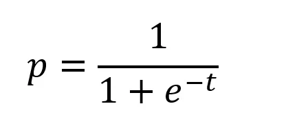
Logistic regression at scale attempts to estimate each prior interaction’s relative impact on an event (usually a sale) by transforming each side of the regression equation with a logarithm. The advantage of this approach over more traditional linear regression is that because the input (independent) and output (dependent) terms are logged, any combination of independent variables is bounded between 0 and 1 (or 0% and 100%). This is also called modeling the log of the odds of an event (the transaction). It is out of the scope of this paper to get into the specifics of how logistic regression (or logit) models works, but suffice to say that the output will be a term for each potential input expressed as a log of the odds, which can be translated to probability with the equation:

Where t is the linear combination:

The trouble with using logistic regression for MTA is that it requires ones (successful sales) and zeros (unsuccessful sales—or potential customers who never became customers.) Unsuccessful sales can be hard to come by. When an entire customer journey is known, for example in the case of a health insurance carrier attempting to get members to take a discrete, known action, this is a very feasible approach. However, when prospective customers don’t have a real defined endpoint, more creative approaches to defining zeroes are needed.
Markov Chain Estimation
The second more advanced approach to parsing value in Markov Chain estimation. This flips logistic regression on its head, and focuses on the upstream tactic—say, clicking an email—and then estimates each next downstream outcome possible from that point. A good visualization of this approach is the old “The Price is Right” game “Plinko.” In this game, the player places a disc at the top of a board with a set of pegs. Each peg represents a random coin flip—so the path that the disc takes is a series of .50 probability decisions resulting in an outcome. However, in Markov Chains, each probability is not 50%–and the disc can end up in more than two next states in the next step.
Markov Chains have the fundamental property of “memorylessness”—their behavior at a given state is only dependent on where they are, not where they have been. This simplifies MTA analysis, but by implication, does not take into account the “saturation” effect of marketing. In other words, we only care that you received a piece of mail at time T, but not how many pieces you received prior to time T. The task of the analyst is to build a matrix of the probabilities of the interaction a customer will have next at a given interaction point, sometimes called a transition probability matrix. For example, this matrix might look like this for an advertiser deploying mainly digital tactics:
| Next State | ||||||||
| Initial | Social | Affiliate | OTT | Sale | No Sale | |||
| Current State | Initial | 0 | 0.40 | 0.20 | 0.30 | 0.10 | 0 | 0 |
| 0 | 0.10 | 0.05 | 0.05 | 0 | 0.01 | 0.78 | ||
| Social | 0 | 0.02 | 0.01 | 0.02 | 0.02 | 0.02 | 0.91 | |
| Affiliate | 0 | 0.04 | 0.01 | 0.03 | 0.01 | 0.03 | 0.88 | |
| OTT | 0 | 0.04 | 0.01 | 0.01 | 0.02 | 0.02 | 0.90 | |
| Sale | 0 | 0 | 0 | 0 | 0 | 1 | 0 | |
| No Sale | 0 | 0 | 0 | 0 | 0 | 0 | 1 | |
The above matrix must meet two conditions:
- Pij is the probability of moving from state i (row, current state) to state j (column, future state); it must also be bounded between 0 and 1 (inclusive)
- The rows (i) have to sum to 1; sale moving to sale is called “absorption” (yes, this is a bit confusing, you can think of it as the journey ending)
From this matrix, it’s possible to calculate the absorption probabilities of each cell—in other words, the probability that at that point, an individual will eventually turn into a sale. To do this, split thetransition matrix into two sub-matrices, Q, the matrix of transitions between non-absorbing states (touchpoints), and R, thematrix of transitions from non-absorbing states to absorbing states (conversion or non-conversion).
Matrix Q:
| Initial | Social | Affiliate | OTT | ||
| Initial | 0 | 0.40 | 0.20 | 0.30 | 0.10 |
| 0 | 0.10 | 0.05 | 0.05 | 0 | |
| Social | 0 | 0.02 | 0.01 | 0.02 | 0.02 |
| Affiliate | 0 | 0.04 | 0.01 | 0.03 | 0.01 |
| OTT | 0 | 0.04 | 0.01 | 0.01 | 0.02 |
Matrix R:
| Sale | No Sale | |
| Initial | 0 | 0 |
| 0.01 | 0.78 | |
| Social | 0.02 | 0.91 |
| Affiliate | 0.03 | 0.88 |
| OTT | 0.02 | 0.90 |
With these two matrices, absorption probabilities are found by calculating the fundamental matrix, F = 1 – Q)-1 where I is the identity matrix and (1 – Q)-1 is the inverse of the matrix I-Q. Finally, multiplying F by R will produce the ultimate probability (absorption) of a sale happening (or not) at any point in the matrix. In the case of the given data, F for “sale” is:
| Next State | |||||
| Social | Affiliate | OTT | |||
| Initial State | 0.011151 | 0.000569 | 0.000587 | 0.000176 | |
| Social | 0.000488 | 0.020235 | 0.000447 | 0.000418 | |
| Affiliate | 0.001401 | 0.000387 | 0.031011 | 0.000324 | |
| OTT | 0.000925 | 0.000256 | 0.000263 | 0.020416 | |
These estimates can then be used to allocate value between touches in a chain. For example, say a user is observed going from email to email to social to OTT, and then finally closing. In this case, the values pulled from the above table would be 0.011151; 0.000569; and 0.000418, with the final step—OTT to absorption—pulled from our first matrix as 0.02. To apportion value, these numbers are summed and divided by the total number of steps in the pathway:
(0.011151 + 0.000569 + 0.000418 + 0.02) = 0.03214
To get to a final contribution vector for each unique journey:
| Touch 1 (Email) | Touch 2 (Email) | Touch 3 (Social) | Touch 4 (OTT) |
| 35% | 2% | 1% | 62% |
Of course, this has to be scaled over thousands and millions of orders—and it’s a lot more complicated than the simple example shown above.
The final question is time. In the example above, say the first interaction (email) happened 90 days ago, but the last interaction before close (Social) was two days ago. Is it fair to give the Email touch 35% credit and the Social touch 1%? Almost certainly not.
There are many techniques for decaying a touch’s impact on ultimate conversion, but they all have the same basic concept: an interaction’s impact fades over time. In MMM (media mix models) we use the term adstock—the rate at which a touch’s “power” decays after it is shown. The concept is similar in MTAs, but is reversed, because we are focused on the sales, not the stimulus. In other words, we look back from the order, not ahead from the stimulus.
The simplest approach for MTA is straight-line decay with a look-back window. This is just as it sounds: A touch before the start of the look-back window gets 0 credit; one mid-way through the window gets ½ of the full credit; and a touch on the day of the order gets full (1) credit. More advanced logistic decay approaches are certainly possible, but yield limited additional benefits and add significant complexity.
Bringing It All Together: How Does Multi Touch Attribution Work?
Putting all of these elements together—the longitudinal human record (LHR), probabilistic inference of non-deterministic touches, estimation of contribution via either logistic regression or Markov Chain analysis, and decay—will give a marketing analytics team the basic elements of multi-touch attribution.
One final, important note: black box MTAs provided by vendors claiming a secret sauce for identity resolution are compelling because they seem simple, but buyer beware. Proprietary identity graphs are only as good as the federations the company belongs to and the underlying cross-walk code, and there is really no way to validate them other than by seeing if they “make sense.” For this reason, they tend to struggle over the long run as accuracy—and hence utility—are questioned by financial decisionmakers. A purpose-built, open-code, white box approach to MTA, which can also be used to power downstream applications like dashboards and econometric MMM panels—should be the preferred approach for marketing analytics teams.

The latest holistic measurement approach: Unified Marketing Measurement
Bring together the strengths of three integrated measurement approaches to make faster, more accurate decisions


